When analysing a dataset, it is useful to be able to say something about interaction between variables. A regression analysis can be used to estimate such a relationship. Such an analysis can be achieved using machine learning. Many packages are available for any programming language to perform linear regression. I decided to write one myself in Python.
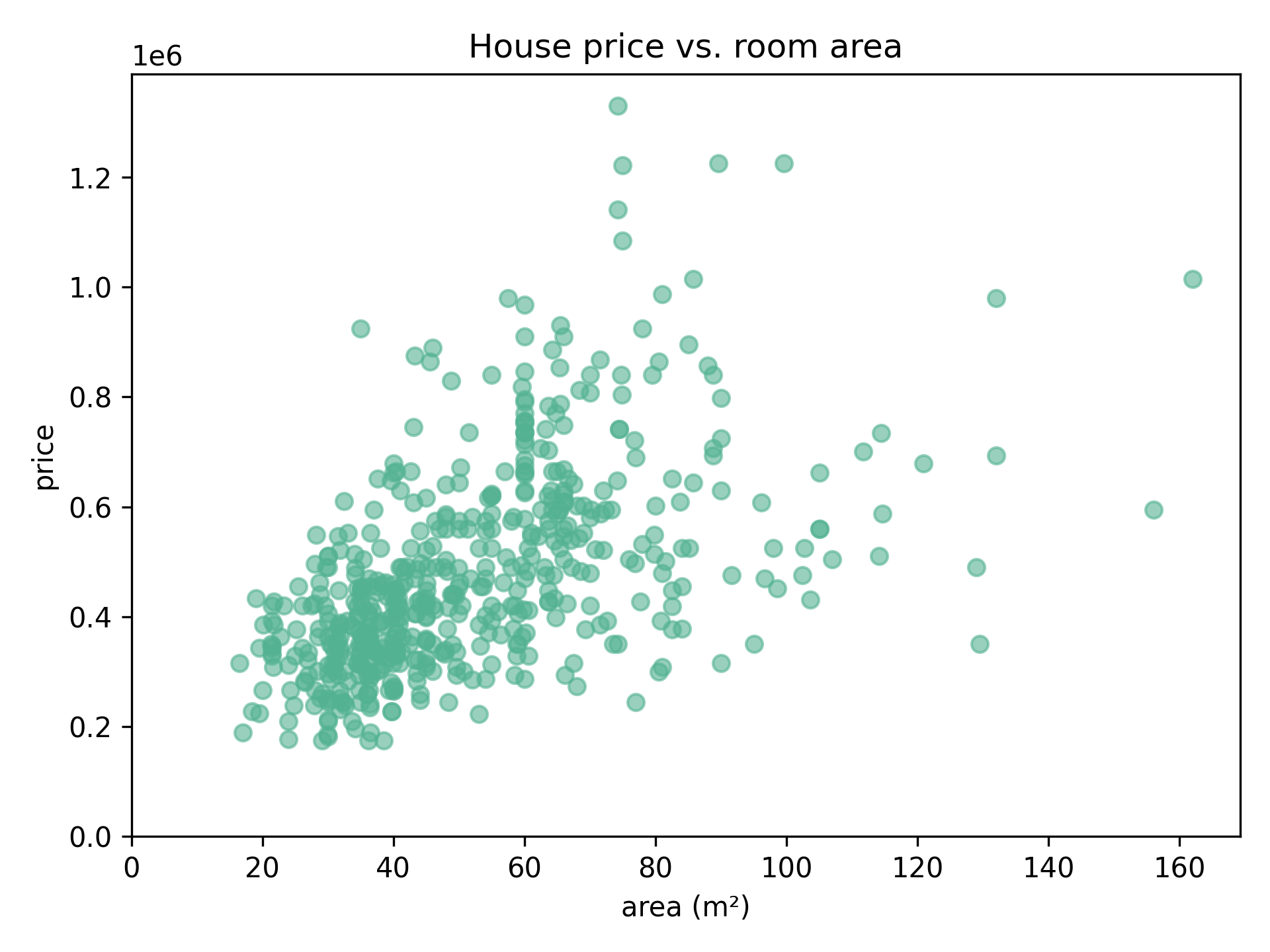
Say we have data on housing prices, and the room area these houses offer. We can plot this data as follows:
Can we say something about how well the area (independent value) can influence the price (dependent value)?
To begin, we can draw a random straight line through the data. We draw this such that $y = ax + b$. In machine learning the a here is also called the weight, and the b is called the bias. Thus, for each value $x$, a $\hat{y}$ value is predicted. Say we start our line 500 000 (the bias), and we take a slope of 1000 (the weight). For every square meter we add to the area, we expect the price to increase by 1000.
# For every x value in the dataset, we can predict a y value using our weight and bias values. By using Numpy this calculation is done for every value automatically.

def predict_y(x: NPArray, weight: float, bias: float) -> NPArray:
    return weight * x + bias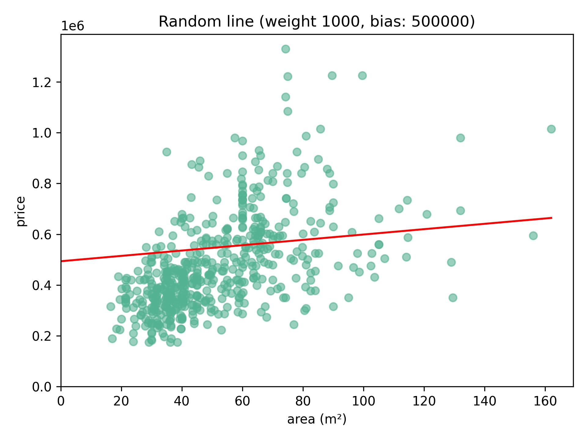
How well does this line fit our data? We can determine this by calculating how far the real values $y$ lay from our approximated values $\hat{y}$ using the line formula. This is called the loss function: $(ŷ - y)^2$. Do this for every data point, and we have a measure of fit: $\frac{1}{2m}\sum\limits_{i=1}^{m} (ŷ_i - y_i)^2$.
def calc_loss(y: NPArray, y_hat: NPArray) -> float:
    loss_array = (y_hat - y) ** 2
    loss: float = np.add.reduce(loss_array) * (1 / (2 * Const.M))
    return loss
Using the loss, we can derive formulas to adjust the weights and biases. This is done by taking the derivative of the loss function above for both.
For the weight: $w_{new} = w - \alpha\frac{1}{m}\sum\limits_{i=1}^{m} (wx_i + b - y_i)x_i$.
For the bias: $b_{new} = b - \alpha\frac{1}{m}\sum\limits_{i=1}^{m} (wx_i + b - y_i)$.
Alpha ($\alpha$) represents the learning rate you want to set. A smaller rate takes longer to compute, but too large a value can result in inaccurate results.
def update_weight(weight: float, bias: float, x: NPArray, y: NPArray) -> float:
    der_array = (weight * x + bias - y) * x
    der = np.add.reduce(der_array) * (1 / Const.M)

    weight_new: float = weight - Const.ALPHA * der
    return weight_new
Repeatedly adjusting the weight and bias 1000 times results in the following line:
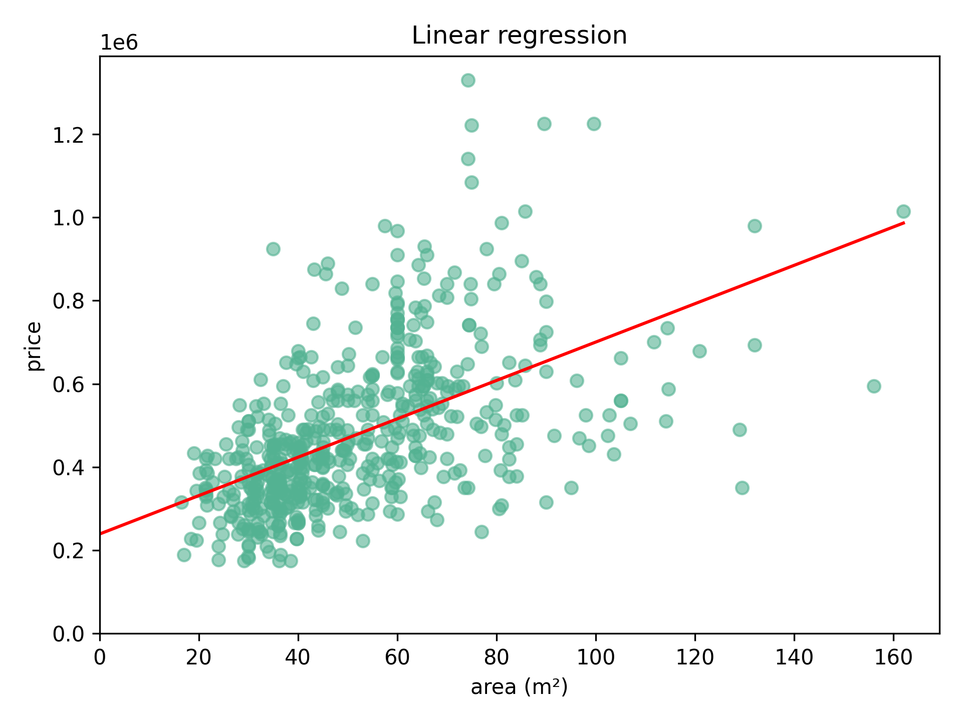
Weight: 4620, bias: 238 733.
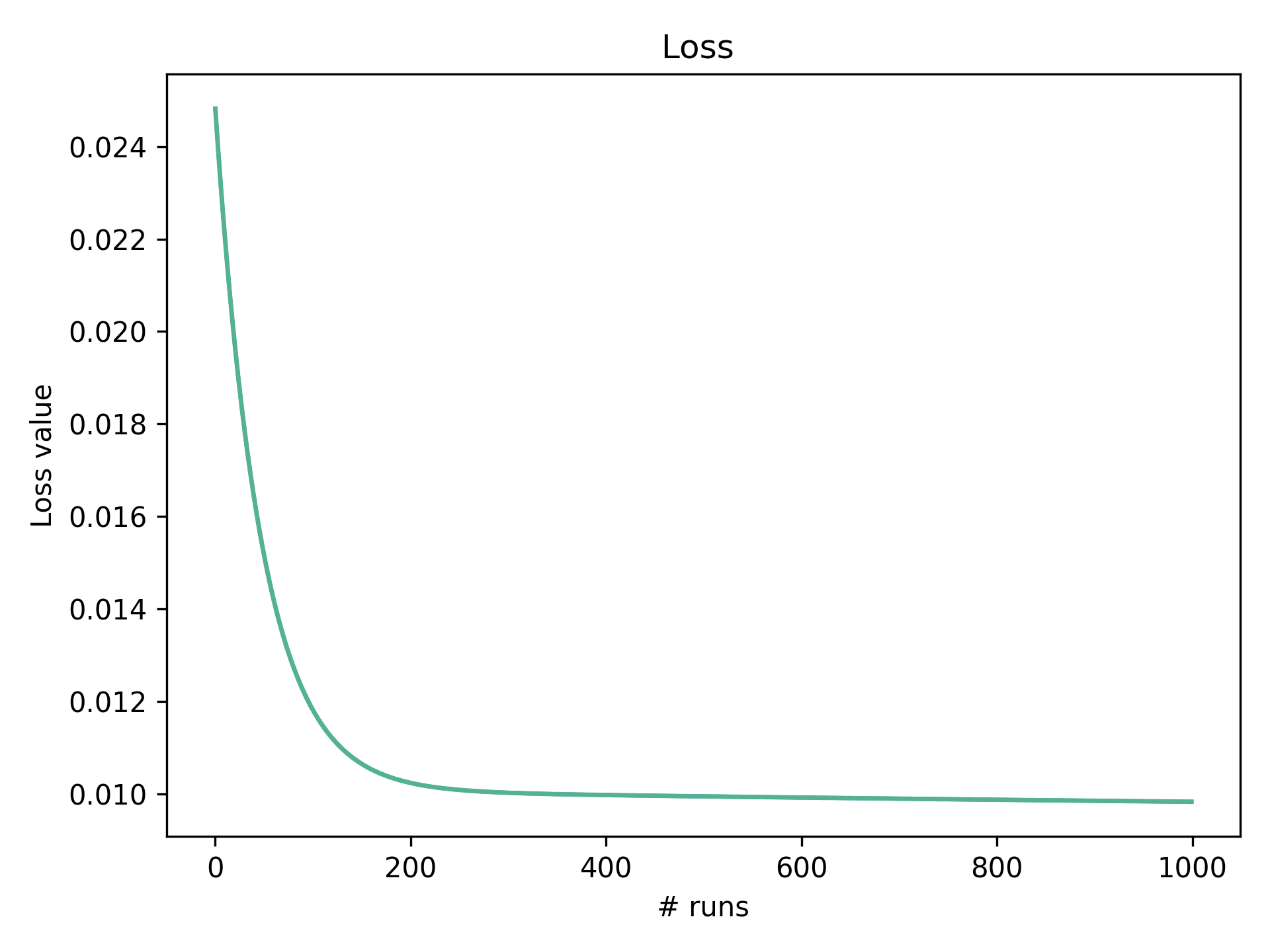
If we plot the loss measure through time we can see as the algorithms repeatedly adjusts the weight and bias (below). The graph converges to the most optimal fit. For this dataset and learning rate, we can see after about 200 runs the loss value starts to flatten. We are now approaching the most optimal line as plotted above.
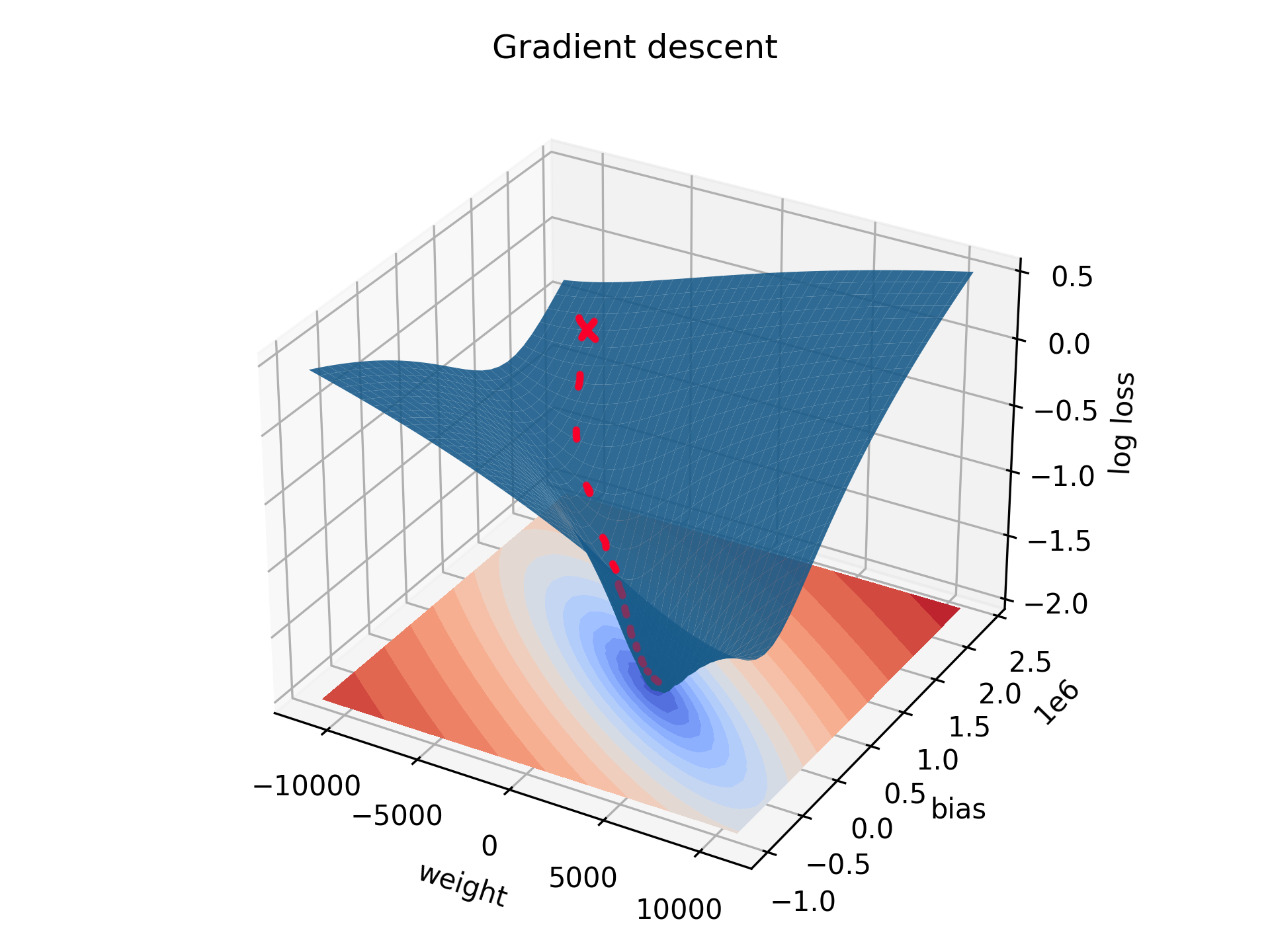
We can also plot this in 3D for a wide variety of possible weights and biases. From whatever starting point (red cross), with enough runs the weight and bias will be adjusted and the loss will decrease accordingly. This is presented as the red line in the graph. Imagine a ball rolling down the slope. This process is called gradient descent. The lowest point on the graph represents the optimal weight and bias we found above.
One form of the loss value that is often reported in a regression analysis is called the R2 value. This is a measure between 0 and 1 on how well the line fits our data. If all data points were to lay on the predicted line, the R would be 1. In our dataset, the R2 value is: 0.29. In other words, 29% of our data can be explained by the line we drew through it.
# The R-squared value can be calculated using the sum of squares total, and sum of squares regression values.

def calc_r_squared(y: NPArray, y_hat: NPArray) -> float:
    sst = np.add.reduce((y-mean(y)) ** 2)
    ssr = np.add.reduce((y_hat-mean(y)) ** 2)

    r_squared = ssr/sst
    return r_squared
Another often used value that is reported is the p-value of the slope. A statistically significant value shows it's likely the slope (weight) is different from zero. In other words, whether there actually exists a relationship between the independent and dependent variables.
In our dataset, the p-value is: 7.40e-42. So very significant.
# The standard error can be calculated using the sum of squares error, the  sum of squares total for x, and the degrees of freedom.
# The t-value can be calculated by dividing the slope by the standard error.
# This value can then be converted to the p-value.

def calc_p_value(y_hat: NPArray, y: NPArray, x: NPArray, weight: float) -> float:
    dof = Const.M - 2
    sse = np.add.reduce((y_hat - y) ** 2)
    x_sst = np.add.reduce((x - mean(x)) ** 2)
    se = sqrt((1 / dof) * (sse / x_sst))
    t_val = weight / se
    p_value: float = t.sf(abs(t_val), dof) * 2  # *2 for two-tailed p-value

    return p_value
Comparing our results to an often used python package Scipy.stats reveals my script to function well.
My script:
Weight: 4619.69
Bias: 238 733.85
R2: 0.2872
p-value: 7.4026e-42
nr. of cycles ran: 5000
Scipy.stats:
LinregressResult(slope=4619.74, intercept=238 730.84)
Scipy.stats r-squared: 0.2872
Scipy.stats p-value: 7.3882e-42
One roadblock in machine learning is the large number of computations that have to be performed. Luckily, we can help the computer via good design of how it handles these calculations. One such aid is found in the popular python package Numpy. Here, computations are performed via vectorization, something the cpu of a computer rather adept at. Using this, calculations across an array can be performed simultaneously and in bulk. The usage of Numpy speeds up certain applications by multiple orders of magnitude.
Computers don't work well with large numbers. Calculation quickly get incredibly large, such as when calculating the loss value using multiplication. To avoid this, we can perform a normalization of the data. For instance, the data in this script was normalized using min-max normalization. Here, the x and y values get normalized between 0 and 1.
# We calculate the upper and lower values of x and y and save them for later.

def normalize_data(x: NPArray, y: NPArray, weight: float, bias: float) -> tuple[NPArray, NPArray]:
    Nor.y_min, Nor.y_max = min(y), max(y)
    Nor.x_min, Nor.x_max = min(x), max(x)

    x_nor = (x - Nor.x_min) / (Nor.x_max - Nor.x_min)
    y_nor = (y - Nor.y_min) / (Nor.y_max - Nor.y_min)
    return x_nor, y_nor
Finally, we can denormalize the data to return the corresponding values in original scale.
# The calculated bounds of before are used again here.

def denormalize_data(x_nor: NPArray, y_nor: NPArray, y_hat: NPArray, weight: float, bias: float) -> tuple[NPNum, NPNum, NPNum, float, float]:
    x = x_nor * (Nor.x_max - Nor.x_min) + Nor.x_min
    y = y_nor * (Nor.y_max - Nor.y_min) + Nor.y_min
    y_hat = y_hat * (Nor.y_max - Nor.y_min) + Nor.y_min
    return x, y, y_hat